A New Modeling Approach

One of the superpowers of Bayesian modeling is that the posterior from a previous run can become the prior for your next run. Until recently I haven’t been utilizing this fact in my hockey model. Silly me, the results of this approach are very effective in allowing the model to respond much more dynamically to changes in team performance, either offensively or defensively.

The original model simply estimated the required parameters from all games in the last 365 days. This is a pretty big assumption: That the innate abilities of the teams are constant over that year long period. Sports fans of any type are eager to incorrectly attribute any small blip in team performance to a permanent change for the better or worse, but I think my old model goes too far in the opposite direction. A year is a long time, and a lot can happen to a team during that span: Traded players, changes in coaching, or a breakdown in synergy on key lines. The new model structure looks like this:

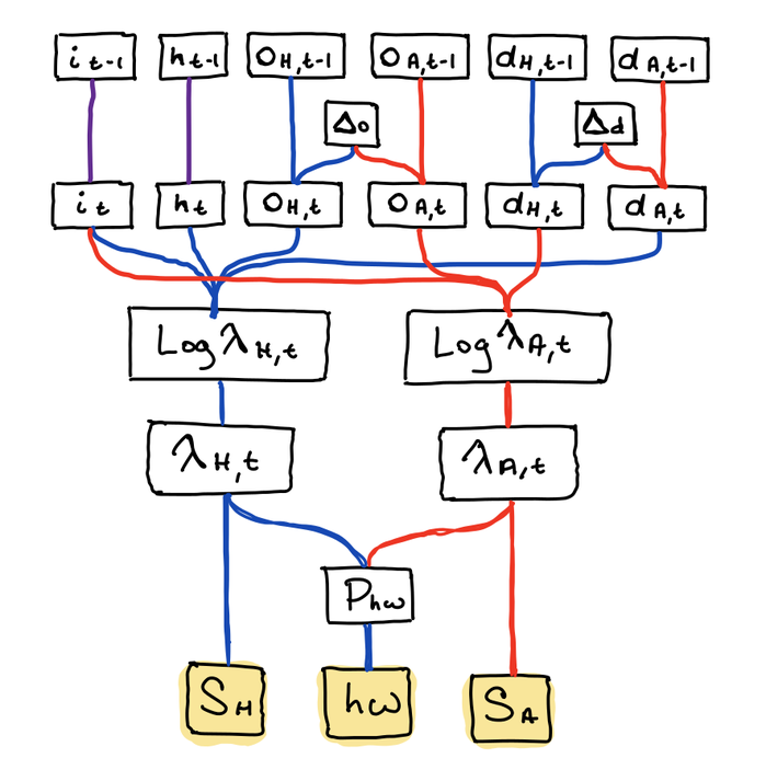
The linkages between parameters are marked by the lines, with red lines corresponding to away team parameters, blue to home team parameters, and purple to league wide parameters. The yellow boxes are the observed random variables for regulation score and whether or not the home team ultimately won. The precise mathematical structure is described in more detail later.

Since the model now considers games played day by day, the priors for each of these daily iterations are simply the posteriors from the previous game day, with a small 2% widening factor applied. This arose out of experimentation and appears to keep the model more open to change. Furthermore, the team offensive and defensive strengths are now explicitly expected to nudge up and down by a small amount each game day. This basically lets each team undergo a small random walk. The idea for this model addition comes from the very excellent book Model-Based Machine Learning by John Winn and his co-authors.

Let’s take a look at the mathematical form. Assume the home team is given an index \(j\) and the away team an index of \(k\). First we have the league wide intercept and home ice advantage parameters:

\[i \sim Normal(\mu_{i,t-1}, \sigma_{i, t-1})\] \[h \sim Normal(\mu_{h, t-1}, \sigma_{h-1})\]

Next there’s the previous game day’s team parameters:

\[o_{j,t-1} \sim Normal(\mu_{o,j,t-1}, \sigma_{d,j,t-1})\] \[d_{j,t-1} \sim Normal(\mu_{o,j,t-1}, \sigma_{d,j,t-1})\] \[o_{k,t-1} \sim Normal(\mu_{o,k,t-1}, \sigma_{d,k,t-1})\] \[d_{k,t-1} \sim Normal(\mu_{o,k,t-1}, \sigma_{d,k,t-1})\]

The random walk adjustments for each team, centered at zero with a small standard deviation:

\[\Delta_o \sim Normal(0, \sigma_{\Delta})\] \[\Delta_d \sim Normal(0, \sigma_{\Delta})\] \[o_{j,t} = o_{j,t-1} + \Delta_o\] \[d_{j,t} = d_{j,t-1} + \Delta_d\] \[o_{k,t} = o_{k,t-1} + \Delta_o\] \[d_{k,t} = d_{k,t-1} + \Delta_d\]

The Poisson/Exponential rate parameters:

\[log\lambda_{H,t} = i + h + o_{j,t} - d_{k,t}\] \[log\lambda_{A,t} = i + o_{k,t} - d_{j,t}\] \[\lambda_{H,t} = exp(log\lambda_{H,t})\] \[\lambda_{A,t} = exp(log\lambda_{A,t})\]

The Poisson distributed regulation time goals for each team:

\[s_{H,t} \sim Poisson(\lambda_{H,t})\] \[s_{A,t} \sim Poisson(\lambda_{A,t})\]

And finally the Bernoulli probability of a home win using the rate parameters under sudden death overtime conditions.

\[p_{hw} = \lambda_{H,t}/(\lambda_{H,t} + \lambda_{A,t})\] \[hw \sim Bernoulli(p_{hw})\]

This model addition makes use of the relationship between Poisson and Exponentially distributed random variables to cast the rate model variables (\(\lambda_{H,t}\) and \(\lambda_{A,t}\)) into a form that predicts the time to next goal for each team. More detail on this in a future blog post!

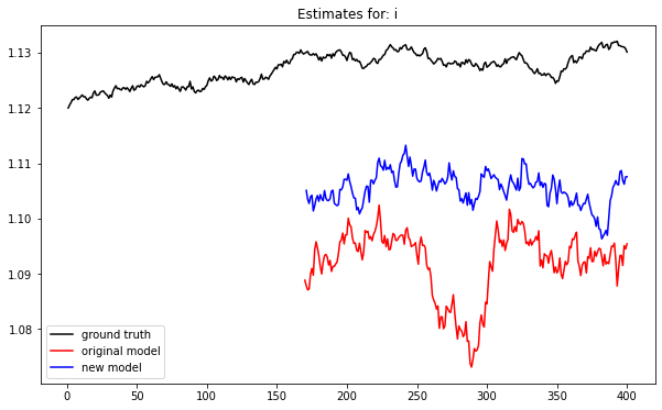
Compared to the old modeling approach, this one yields better inference of the latent parameters when executed on an ideal data generation process that approximately mirrors NHL scheduling. For example here the model is estimating the intercept parameter \(i\) on ideal simulated data:

And for the parameter \(h\) we have:

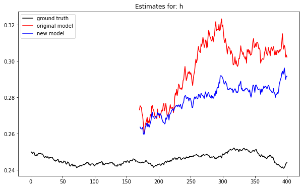
For both models the parameter \(i\) is underestimated while \(h\) is over estimated. But clearly the new model is closer to the truth. Across all of the latent variables the MSE of estimates for the old model fit is 0.00441 while it’s 14% lower at 0.00379 for the new model.

Making Posteriors into Priors

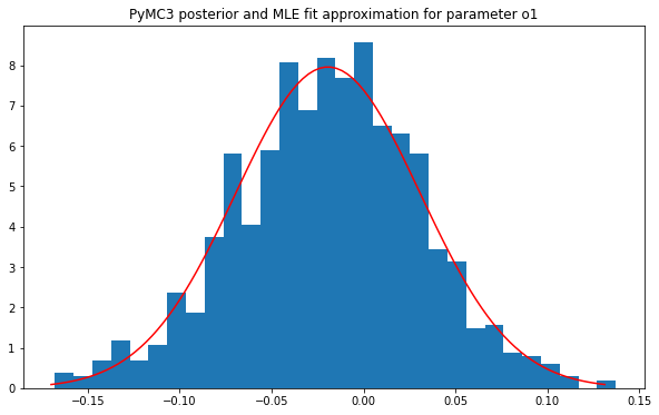
Of course a MCMC based Bayesian estimation framework like PyMC3 doesn’t actually give you a proper probability distribution as a posterior; you actually get a trace for the parameter, which is just a sample whose density approximates the true posterior. In this form you can’t just plug it into the model for the next run. To handle this, I leverage SciPy to find the maximum likelihood estimate (MLE) of the ideal probability distribution for each parameter in the trace. This is what gets plugged in as the priors for the next iteration. It works because the posterior density from PyMC3 for one of the originally normal model parameters is generally pretty close to normal itself. For example, here is the MLE fit and a histogram of the actual PyMC3 posterior for the team one’s offence after the first model iteration:

A secondary benefit of this new approach to handling posteriors is that I can store these MLE fit distributions directly and use them to compute arbitrary game outcomes and score distributions for the future. This allows me to forgo the old approach of storing thousands of simulated games in PostgreSQL and opens up new possibilities for simulating hypothetical games selected by the user on any given game date. I hope to add this as a feature to the web app https://bayesbet.everettsprojects.com/ at a later date.

I also took advantage of the lower storage required by this approach to move the model parameters and game predictions into DynamoDB. Since I’m using on the on demand version of the service and have low traffic, this saves me the $13 a month that I was spending on AWS’s RDS service before.

Watch out for a future series of posts tht will explore the mathematics behind computing goal distributions and game outcomes from these new posterior distributions in more detail.