Is Home Ice Advantage in the NHL Real?
Many people have attempted to answer the question of whether or not home ice advantage exists. A 2013 paper by Tim Swartz and Adriano Arce came to the conclusion that home ice advantage in the NHL is real, accounting for about 5% of goals in 2012. Furthermore, they observed that when total goals per game are accounted for, there is no appreciable change in the home ice advantage over time. Lastly, they performed a one way ANOVA and a pairwise Tukey’s HSD test on 16 NHL teams that have played in 30 seasons to determine if there is a significant difference between teams’ home ice advantages. The result from their analysis was that there is not sufficient evidence to conclude that home ice advantage varies between teams.
Later in 2017, a fivethirtyeight blog post also tried to tackle this problem, coming to the conclusion that home ice in the regular season amounts to a win percentage of 55.1%, 5.1% better than even odds. In the playoffs this advantage declines slightly to a boost in win percentage that is only 4.8% better on home ice than at a theoretical neutral rink.
The above two results appear fairly consistent with each other, and one might be satisfied that home ice advantage is a real phenomenon. This is probably a safe bet, but I’m all for reproducible research so I’m going to try my hand at answering this question myself and corroborating the previous findings. My goal is also to learn a bit about the nature of home ice advantage so I can use it later in a model for predicting NHL game outcomes.
There are three questions that I want to answer:
- Is there evidence for home ice being advantageous in general?
- Is there evidence that this advantage varies from team to team?
- Is there evidence that home ice advantage still exists if a game goes to overtime or shootout?
To do all of this I am going to a use few different strategies. First I will attempt to demonstrate that the distribution of goal totals for home and away teams follow a Poisson distribution. Then I will show that the distributions are significantly different using a Wilcoxon Signed-Rank Test. Next, I will try to determine if the extent of home ice advantage varies significantly from team to team using a two way ANOVA on a Poisson Generalized Linear Model. Finally, I will look at whether there is evidence for home ice advantage still playing a role in games that go to overtime or shootout using binomial tests and a simple proportion test.
Overall the analysis I am about to do will be fairly quick and dirty, because I’m really only interested in answering the above questions to guide my model building process for my next post. As such, I do not recommend that anyone take the results of this analysis as being authoritative.
Acquiring Official NHL Data
To start, we will need to get the data for NHL games that have already been played. I will do this using the undocumented NHL statistics API, which returns json files with a mostly self evident structure. These files will be retrieved and parsed using Python and the very easy requests and json libraries.
import requests
import json
import pandas as pd

base_url = "https://statsapi.web.nhl.com"
schedule_path = "/api/v1/schedule?startDate=2013-09-18&endDate=2017-08-1&expand=schedule.linescore"
schedule_response = requests.get(base_url + schedule_path)
schedule_json = schedule_response.json()

# A function to extract the relevant data from the schedule
# and return it as a pandas dataframe
def extract_game_data(schedule):
    """Given full JSON records for games from the NHL API,
    returns a simplified list of just the data we need.
    """
    games = pd.DataFrame(columns=['date',
                                  'season',
                                  'game_type',
                                  'home_team',
                                  'home_team_reg_score',
                                  'home_team_fin_score',
                                  'away_team',
                                  'away_team_reg_score',
                                  'away_team_fin_score',
                                  'went_to_shoot_out'
                                  ])

    for date_obj in schedule_json['dates']:
        date = date_obj['date'];
        for game_obj in date_obj['games']:
            game_type = game_obj['gameType']
            season = game_obj['season']
            home_team_obj = game_obj['teams']['home']
            away_team_obj = game_obj['teams']['away']

            home_team = home_team_obj['team']['name']
            home_team_fin_score = home_team_obj['score']

            away_team = away_team_obj['team']['name']
            away_team_fin_score = away_team_obj['score']

            detailed_score_data = game_obj['linescore']
            period_data = detailed_score_data['periods']
            shootout_data = detailed_score_data['shootoutInfo']

            home_team_reg_score = 0
            away_team_reg_score = 0

            for period in period_data[0:3]:
                home_team_reg_score += period['home']['goals']
                away_team_reg_score += period['away']['goals']

            went_to_shoot_out = (shootout_data['home']['attempts'] != 0 or
                                 shootout_data['away']['attempts'] != 0)

            games = games.append({'date': date,
                                  'season': season,
                                  'game_type': game_type,
                                  'home_team': home_team,
                                  'home_team_reg_score': home_team_reg_score,
                                  'home_team_fin_score': home_team_fin_score,
                                  'away_team': away_team,
                                  'away_team_reg_score': away_team_reg_score,
                                  'away_team_fin_score': away_team_fin_score,
                                  'went_to_shoot_out': went_to_shoot_out
                                  }, ignore_index=True)

    return games

games = extract_game_data(schedule_json)
games.to_csv('games.csv', index = False)
Are the Distributions of Regulation Time Goals Poisson?
Let’s start by looking at the actual distribution of home and away goals.
library(tidyverse)
library(lubridate)

games <- read_csv("games.csv")

reg_season_games <- games %>%
  filter(game_type == "R")
dim(reg_season_games)
## [1] 4920 10home_actual_score_counts <- reg_season_games %>% count(home_team_reg_score)
away_actual_score_counts <- reg_season_games %>% count(away_team_reg_score)
actual_score_counts <- reg_season_games %>%
select(home_team_reg_score, away_team_reg_score) %>%
gather(key = game_type, value = goals, home_team_reg_score, away_team_reg_score) %>%
count(game_type, goals) %>%
rename(game_count = n)
actual_score_counts %>%
ggplot() +
geom_col(aes(x = goals, y = game_count, fill = game_type), position = "dodge") +
scale_x_continuous(breaks = seq(0, 10, by = 1)) +
scale_fill_manual(labels = c("Away", "Home"), values = c("#F8766D", "#00BFC4")) +
labs(title = "Distribution of Actual Goals",
x = "Goals Scored in Game",
y = "Game Count",
fill = "Team Type")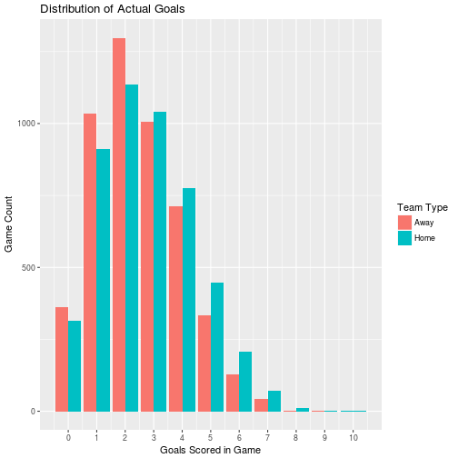
Both appear to be roughly Poisson distributed at first glance. Next let’s look at how the observed home and away goal distributions compare to a theoretical Poisson distribution with the same mean.
home_actual_score_counts <- reg_season_games %>% count(home_team_reg_score)
away_actual_score_counts <- reg_season_games %>% count(away_team_reg_score)

home_expected_score_probs <- dpois(home_actual_score_counts$home_team_reg_score, lambda = mean(reg_season_games$home_team_reg_score))
home_expected_score_comp <- 1.0- sum(home_expected_score_probs)

away_expected_score_probs <- dpois(away_actual_score_counts$away_team_reg_score, lambda = mean(reg_season_games$away_team_reg_score))
away_expected_score_comp <- 1.0 - sum(away_expected_score_probs)
Home:
chisq.test(x = c(home_actual_score_counts$n, 0), p = c(home_expected_score_probs, home_expected_score_comp), simulate.p.value = TRUE)##
## Chi-squared test for given probabilities with simulated p-value
## (based on 2000 replicates)
##
## data: c(home_actual_score_counts$n, 0)
## X-squared = 26.521, df = NA, p-value = 0.01249home_score_count_comparisons <- actual_score_counts %>%
filter(game_type == "home_team_reg_score") %>%
rename(actual = game_count) %>%
mutate(expected = nrow(reg_season_games) * dpois(goals, lambda = mean(reg_season_games$home_team_reg_score))) %>%
gather(key = count_type, value = count, actual, expected) %>%
count(goals, count_type, count) %>%
rename(game_count = count)
home_score_count_comparisons %>%
ggplot() +
geom_col(aes(x = goals, y = game_count, fill = count_type), position = "dodge") +
scale_x_continuous(breaks = seq(0, 10, by = 1)) +
labs(title = "Distribution of Actual and Expected Goals for Home Teams",
x = "Goals Scored in Game",
y = "Game Count",
fill = "Observation Type")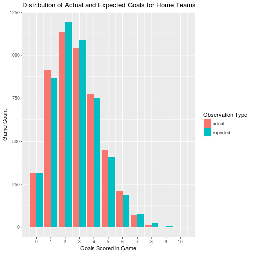
Away:
chisq.test(x = c(away_actual_score_counts$n, 0), p = c(away_expected_score_probs, away_expected_score_comp), simulate.p.value = TRUE)##
## Chi-squared test for given probabilities with simulated p-value
## (based on 2000 replicates)
##
## data: c(away_actual_score_counts$n, 0)
## X-squared = 26.946, df = NA, p-value = 0.004998away_score_count_comparisons <- actual_score_counts %>%
filter(game_type == "away_team_reg_score") %>%
rename(actual = game_count) %>%
mutate(expected = nrow(reg_season_games) * dpois(goals, lambda = mean(reg_season_games$away_team_reg_score))) %>%
gather(key = count_type, value = count, actual, expected) %>%
count(goals, count_type, count) %>%
rename(game_count = count)
away_score_count_comparisons %>%
ggplot() +
geom_col(aes(x = goals, y = game_count, fill = count_type), position = "dodge") +
scale_x_continuous(breaks = seq(0, 10, by = 1)) +
labs(title = "Distribution of Actual and Expected Goals for Away Teams",
x = "Goals Scored in Game",
y = "Game Count",
fill = "Observation Type")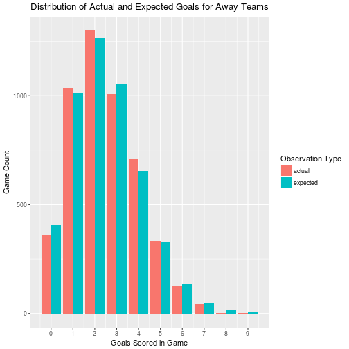
We can see that the distribution of scores for both home and away teams is not actually Poisson, but it pretty close. I appears to skew slightly lower than the expected values, which means the data is under-dispersed. This under-dispersion doesn’t appear to be very severe however, so I am comfortable going forward assuming that the goal counts can be modeled as Poisson.
Is There a Difference Between Home and Away Goal Counts?
Because our distributions are not even remotely normal, but also not exactly Poisson, I will use the Wilcoxon Signed Rank Test to test if the means of each are different:
wilcox.test(reg_season_games$home_team_reg_score,
            reg_season_games$away_team_reg_score,
            paired = TRUE,
            conf.level = 0.95)
##
## Wilcoxon signed rank test with continuity correction
##
## data: reg_season_games$home_team_reg_score and reg_season_games$away_team_reg_score
## V = 3994200, p-value = 7.028e-14
## alternative hypothesis: true location shift is not equal to 0The Wilcoxon Signed Rank Test has yielded a highly significant p-value. This indicates that the average score differential of 0.252 additional goals for the home team is a real effect, not just statistical noise.
Does Home Ice Advantage Vary by Team?
In order to assess if the interaction between team and home vs away games is significant, I will run an ANOVA on a Poisson family generalized linear model fit to the goal data from each game. My intent with this is to use the interaction term to decide if there is evidence that home team advantage varies by team.
reg_season_games_home <- reg_season_games %>%
  select(home_team, home_team_reg_score) %>%
  rename(team = home_team, goals = home_team_reg_score) %>%
  mutate(game_type = "home")

reg_season_games_away <- reg_season_games %>%
  select(away_team, away_team_reg_score) %>%
  rename(team = away_team, goals = away_team_reg_score) %>%
  mutate(game_type = "away")

reg_season_games_for_anova <- rbind(reg_season_games_home, reg_season_games_away)
poisson_glm <- glm(goals ~ team * game_type, family = poisson, data = reg_season_games_for_anova)
summary(aov(poisson_glm))## Df Sum Sq Mean Sq F value Pr(>F)
## team 30 446 14.88 6.005 <2e-16 ***
## game_type 1 157 156.76 63.277 2e-15 ***
## team:game_type 30 64 2.13 0.860 0.685
## Residuals 9778 24224 2.48
## ---
## Signif. codes: 0 '***' 0.001 '**' 0.01 '*' 0.05 '.' 0.1 ' ' 1In the above Two Way ANOVA, we can see that the effect of team on goals scored is highly significant, as is the effect of game_type. This means that the mean number of goals scored per game varies between home and away games when we ignore which teams were playing. We already determined this earlier with the Wilcoxon Signed Rank Test, so it is reassuring to see the same result here. Similarly, the mean number of goals scored per game varies between teams when ignoring if a game was played at home or away. The interaction term has a p-value of 0.648, which is no where near to being significant. This indicates to us that there is insufficient evidence to conclude that the effective difference between home and away games varies across teams. This appears to answer our second question with a definitive “no”.
Does Home Ice Advantage Exist in Overtime or Shoot Out?
Finally, we will attempt to answer one last question: Does the home team still have an advantage if a game goes to overtime? To answer this question I will split the games into two categories for overtime wins, and non-overtime wins. I will then examine if there is evidence that either of these differ from even odds. Finally I will use R’s prop.test() function to see if there is evidence that the two proportions differ.
reg_season_games_wins <- reg_season_games %>%
  mutate(home_win = home_team_fin_score > away_team_fin_score) %>%
  mutate(OT_win = home_team_reg_score == away_team_reg_score)

reg_season_games_wins %>% group_by(OT_win) %>% summarize(mean_home_wins = mean(home_win), n = n())
## # A tibble: 2 x 3
## OT_win mean_home_wins n
## <lgl> <dbl> <int>
## 1 F 0.552 3743
## 2 T 0.510 1177non_ot_home_wins <- reg_season_games_wins$home_win[reg_season_games_wins$OT_win == FALSE]
ot_home_wins <- reg_season_games_wins$home_win[reg_season_games_wins$OT_win == TRUE]
x1 <- sum(non_ot_home_wins)
n1 <- length(non_ot_home_wins)
x2 <- sum(ot_home_wins)
n2 <- length(ot_home_wins
)
binom.test(x1, n1, 0.5)##
## Exact binomial test
##
## data: x1 and n1
## number of successes = 2065, number of trials = 3743, p-value =
## 2.707e-10
## alternative hypothesis: true probability of success is not equal to 0.5
## 95 percent confidence interval:
## 0.5355956 0.5677166
## sample estimates:
## probability of success
## 0.5516965binom.test(x2, n2, 0.5)##
## Exact binomial test
##
## data: x2 and n2
## number of successes = 600, number of trials = 1177, p-value =
## 0.5214
## alternative hypothesis: true probability of success is not equal to 0.5
## 95 percent confidence interval:
## 0.4807925 0.5386998
## sample estimates:
## probability of success
## 0.5097706We can see that there is evidence for home ice advantage leading to wins during regulation time, but once a game goes to overtime the evidence in favour of home ice advantage appears to vanish.
prop.test(x = c(x1, x2), n = c(n1, n2))##
## 2-sample test for equality of proportions with continuity
## correction
##
## data: c(x1, x2) out of c(n1, n2)
## X-squared = 6.1721, df = 1, p-value = 0.01298
## alternative hypothesis: two.sided
## 95 percent confidence interval:
## 0.008664835 0.075186958
## sample estimates:
## prop 1 prop 2
## 0.5516965 0.5097706Running a proportion test confirms that the two proportions appear to be different. For the purposes of my hierarchical Bayesian model, I will assume that once a game goes to overtime the probability of one team winning over the other will just be a Bernoulli random variable with probability based on the historical win percentage of that team over the other. No home ice advantage will be considered at that point.