A Bayesian Analysis of My D&D Dice
Shiny App
Test your own dice using this shiny app: https://evjrob.shinyapps.io/bayesian-dnd/
Introduction
My girlfriend and I have been attending a weekly Dungeons & Dragons night at a local board game cafe, which means that we have been thoroughly immersed in the superstition surrounding the dice. We have heard stories of unlikely strings of bad rolls that ultimately lead to the frustrated fellow adventurer performing the salt water test to see if the dice are balanced poorly. This test is really cool, and it certainly explains the physical mechanism for why a die will come up on some faces more than others, but it doesn’t tell you anything about the probabilities of rolling each face. Even with an off balance die, say a d20 that’s weighted in favour of rolling a twenty, we shouldn’t expect every normal roll on a hard surface to come up twenty. How frequently it comes up will presumably depend on the severity of the balance issue. As an aspiring data scientist I couldn’t help but think that a much better approach would be a Bayesian analysis for estimating the probability of rolling each face.
Normally I don’t care too much about such superstitions and just take the rolls as they come. I probably never would have implemented this Bayesian analysis, if not for the fact that I have developed a bit of a reputation for rolling high damage numbers on my d10 at our table. The curiosity has now gotten the better of me and I want to know the truth about how my dice really roll.
Methodology
There are a couple different ways I can think of to assess if my dice are correctly balanced. I could always use a simple frequentist hypothesis test and set a null hypothesis of p being equal to the fair probability for each face. I could then roll the dice many times and see if the observed data provides enough evidence to reject that hypothesis that the dice is fair. This is a nice and simple approach, which would be straight forward to test using the multinomial or binomial distribution. But there are a couple of drawbacks to this approach that I can immediately think of:
- It tells us nothing about what a better estimate of the probability for each face is; and
- We will likely need a lot more data to achieve significance using this frequentist approach.
Instead, I think a Bayesian approach will be much more informative. We have a couple options available to us: We can use a numerical approach like MCMC, and compute the posterior distributions for each face that way. Or we can try to find an analytically tractable way of computing the posterior from our prior and our observations. Generally this only occurs when we are lucky enough to have a prior and observations of specific forms that allow to easily compute the posterior, a mathematical feature called conjugacy. Luckily for us, there are two useful cases of conjugacy for us to consider. They are the beta-binomial model, and the more general Dirichlet-multinomial model. Ultimately both will be used in this analysis.
The Dirichlet-multinomial model allows us to model an n-dimensional system of discrete events with varying probabilities that all sum to one. Essentially a dice. The beta-binomial model is a special case of the Dirichlet-multinomial model in which n = 2, and it basically describes a coin. Let’s cover the simpler beta distribution and the beta-binomial model before going into the more general Dirichlet distribution and Dirichlet-multinomial model.
Starting with the binomial distribution, the probability mass function is simply:
\[\frac{n!}{k!(n-k)!} p^k(1-p)^{n-k}\]Where n is the total number of trials, k is the number of successes, and p is the probability of a success. It is just a way of determining the probability of observing k heads or tails on n coin flips, and he sum of the probabilities for k from 0 to n is simply 1. For a fair coin the binomial distribution of 20 coin flips looks like:
binom_data <- tibble(k = c(0:20), prob = dbinom(x = c(1:20), size = 20, prob = rep(0.5,21)))

ggplot(data = binom_data) +
  geom_col(aes(x = k , y = prob)) +
  labs(title = "Binomial Distribution for Twenty Coin Flips",
       x = "k Successes",
       y = "Probability of Observing k Successes") +
  theme(legend.position="none")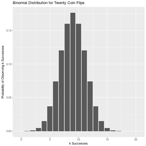
This presumes that we already know the true probability for p. In our case we are uncertain about the probability, so how do we deal with that? This is where the beta prior in the beta-binomial model comes in handy. In our Bayesian approach we get to start with a prior belief of what the probability of rolling a specific face of the coin is. Rather than picking a single value like we would in frequentist statistics, we define a probability density function that shows our relative belief in any p being true across all possible values of p. Since we are working with a probability, this is the range 0 to 1. Using observed data of k successes in n trials, we can update the beta prior distribution to find our posterior distribution. This is all a result of conjugacy, which is just a fancy way of saying that if we start with a beta distribution for the probability p, and then gather data that comes from a binomial distribution, we can find a new beta distribution that describes the posterior probability of seeing that face.
I will skip the math that goes into the beta-binomial model and just assert that this rule for updating the probability distribution from the prior to the posterior is simply:
\[Prior = Beta(\alpha 0,\beta 0)\] \[Posterior = Beta(\alpha 0 + successes,\beta 0 + failures)\]Where $\alpha 0$ and $\beta 0$ are parameters of our prior beta distribution, successes is the number of times we saw our chosen face, and failures is the number of times we didn’t see that face.
Before we get started we need to determine a reasonable beta prior to use. Let’s consider the analysis of a twenty sided dice for the rest of this section, where were are interested in only the probability of rolling a given face, say twenty. All other faces will be lumped together as not twenty so we can still work with the beta distribution. If we honestly knew nothing about dice, we might decide that any value of p is just as likely as the rest, and assign a uniform prior distribution. This can be achieved with $Beta(1,1)$:
ggplot(data.frame(x = c(0:1))) +
  stat_function(fun = dbeta,
                args = list(shape1 = 1, shape2 = 1)) +
  stat_function(fun = dbeta,
                args = list(shape1 = 1, shape2 = 1),
                xlim = c(0,1),
                geom = "area",
                aes(x, alpha = 0.5)) +
  labs(title = "Beta(1,1) Distribution",
       x = "Binomial probability, p",
       y = "Probability density of p") +
theme(legend.position="none")-1.png)
But we do know a little bit about how dice work, and usually our prior belief in the likelihood of any given face is based on the dice being fair. For our d20, this means we expect p = 0.05. To model this prior we could simply say that we expect 1 roll out of twenty to be our face, and model it with $Beta(1,19)$:
ggplot(data.frame(x = c(0:1))) +
  stat_function(fun = dbeta,
                args = list(shape1 = 1, shape2 = 19)) +
  stat_function(fun = dbeta,
                args = list(shape1 = 1, shape2 = 19),
                xlim = c(0,1),
                geom = "area",
                aes(x, alpha = 0.5)) +
  labs(title = "Beta(1,19) Distribution",
       x = "Binomial probability, p",
       y = "Probability density of p") +
theme(legend.position="none")-1.png)
Notice that this isn’t a very confident prior distribution. We can see a decent likelihood for values of p anywhere between 0 and 0.25. If we want a stronger prior we can use larger values of $\alpha$ and $\beta$ where $\frac{\alpha}{(\alpha + \beta)} = 0.05$. Let’s look at $Beta(5,95)$:
ggplot(data.frame(x = c(0:1))) +
  stat_function(fun = dbeta,
                args = list(shape1 = 5, shape2 = 95)) +
  stat_function(fun = dbeta,
                args = list(shape1 = 5, shape2 = 95),
                xlim = c(0,1),
                geom = "area",
                aes(x, alpha = 0.5)) +
  labs(title = "Beta(5,95) Distribution",
       x = "Binomial probability, p",
       y = "Probability density of p") +
theme(legend.position="none")-1.png)
That’s a bit better. There is a definite peak around p = 0.05 with a much tighter spread. You may find it strange that we are going through all this effort just to maintain uncertainty about the value of p. Isn’t our goal to get more confident in the true probability of rolling a certain face? It seems counter intuitive, but the power of Bayesian statistics is that we can continually work with uncertainty in our estimates, and that we treat p as a probability density function rather than a point estimate. This is true in both the prior and the posterior. Think of it as a means of not just finding a new most likely value for p, but also finding our uncertainty in this estimate of p, so that we also know how confident we are in our new estimate. If we wanted to find some common summary statistics for p from a beta distribution (either the prior or the posterior), we can do it with the following formulas and functions:
\[Mean = \frac{\alpha}{\alpha + \beta}\] \[Median = qbeta(0.5, \alpha, \beta)\] \[Mode = \frac{\alpha - 1}{\alpha + \beta -2}\]More important than these summary statistics, however, is our ability to calculate a credible interval for the beta distribution. This gives us something similar to a frequentist confidence interval, except that we can actually say there is a certain probability that the interval contains the true value of p given our assumptions (our prior). Much like the median, the credible interval can be found by passing the appropriate quantiles to the qbeta function for our posterior. For a 95% credible interval, these would be 0.025 for the lower bound an 0.975 for the upper bound.
To solidify all of this with an example, let’s consider our d20 dice after we rolled an unfortunate series of ones that finished off our unfortunate hero. We believe that the dice is fair, and we are interested in determining the posterior probability of rolling a one on it to verify this. We start with a beta(5,95) distribution as our prior and we roll the dice 100 times. In these hundred rolls, we observe a one twenty times, and faces other than a one for the remaining 80 times. Using the beta-binomial updating rule, our posterior is simply:
\[Posterior = Beta(5 + 20,95 + 80) = Beta(25,175)\]And the mean of this posterior distribution is:
\[Mean = \frac{\alpha}{\alpha + \beta} = \frac{25}{25 + 175} = 0.125\]Notice that because we had a prior equivalent to 100 points of data, and collect another 100 points of data to update it, that the new posterior is right in the middle of our prior of p = 0.05 and our observed proportion of 0.20.
Plotting the prior and posterior distributions together, we can see this shift:
ggplot(data.frame(x = c(0:1))) +
  stat_function(fun = dbeta,
                args = list(shape1 = 5, shape2 = 95),
                color = "blue") +
  stat_function(fun = dbeta,
                args = list(shape1 = 5, shape2 = 95),
                xlim = c(0,1),
                geom = "area",
                aes(x, alpha = 0.5),
                fill = "blue") +
  stat_function(fun = dbeta,
                args = list(shape1 = 25, shape2 = 175),
                color = "red") +
  stat_function(fun = dbeta,
                args = list(shape1 = 25, shape2 = 175),
                xlim = c(0,1),
                geom = "area",
                aes(x, alpha = 0.5),
                fill = "red") +
  labs(title = "Beta(5,95) Prior Distribution and Beta(25,175) Posterior Distribution",
       x = "Binomial probability, p",
       y = "Probability density of p") +
  theme(legend.position="none")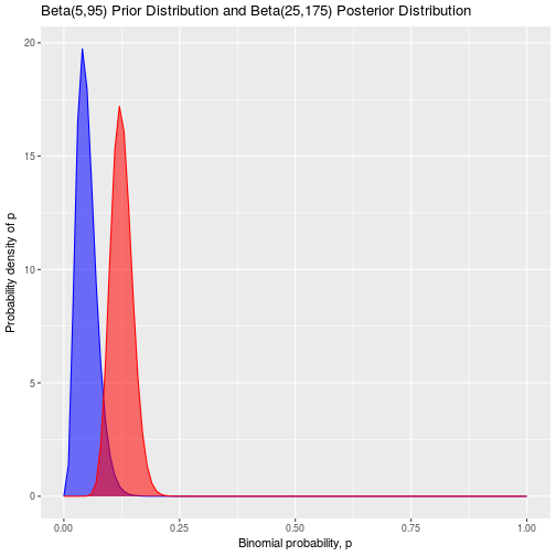
Notice that the high observed frequency of rolled ones has really shifted the distribution for the probability upwards from p = 0.05. It has also widened our posterior distribution compared to our prior, because we are less certain about the probability of rolling a one after such an unexpected result on 100 rolls. A nice feature of Bayesian statistics is is that we can take a posterior distribution and use it as our new prior while we continue testing and collecting more data. Let’s pretend that after seeing this result we are not satisfied, so we decide to roll the dice 1000 more times and observe 203 ones:
\[Posterior = Beta(25 + 203,175 + 797) = Beta(228,972)\] \[Mean = \frac{228}{228 + 972} = 0.190\]ggplot(data.frame(x = c(0:1))) +
stat_function(fun = dbeta,
args = list(shape1 = 25, shape2 = 175),
color = "blue") +
stat_function(fun = dbeta,
args = list(shape1 = 25, shape2 = 175),
xlim = c(0,1),
geom = "area",
aes(x, alpha = 0.5),
fill = "blue") +
stat_function(fun = dbeta,
args = list(shape1 = 228, shape2 = 972),
color = "red") +
stat_function(fun = dbeta,
args = list(shape1 = 228, shape2 = 972),
xlim = c(0,1),
geom = "area",
aes(x, alpha = 0.5),
fill = "red") +
labs(title = "Beta(25,792) Prior Distribution and Beta(228,972) Posterior Distribution",
x = "Binomial probability, p",
y = "Probability density of p") +
theme(legend.position="none")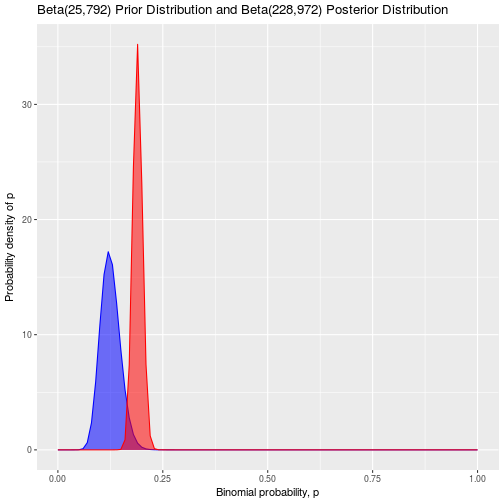
The posterior distribution has narrowed, and the mean has moved further towards the right to p = 0.190. This illustrates another useful feature of Bayesian statistics: As we collect more data, our chosen prior has less influence and becomes less important.
This is how the beta-binomial model works when we only care about one face, but what about if we are interested in every face of the dice? To answer that, let’s look at the Dirichlet distribution and the Dirichlet-multinomial model. We will consider a made up dice that only has three faces, because it will be very difficult to visualize anything higher.
The multinomial distribution is just a higher dimension version of the binomial distribution. In a binomial distribution the probability of a failure can be inferred from the probability of a success since there is a constraint that both outcomes must sum to a total probability of 1. In the multinomial we no longer have success and failure, but outcomes 1,2,…,k each with their own probabilities, $p_i$:
\[f(x_1,...,x_k, p1,...,pk) = \frac{n!}{x_1! x_2! ... x_k!}p_1^{x_1}p_2^{x_2} ... p_k^{x_k}\]Subject to the constraints:
\[\sum_{i=1}^{n} x_i = n\]and
\[\sum_{j=1}^{k} p_j = 1\]Hopefully the similarity of the multinomial model to the binomial model is evident, but if not, then the similarity between the Dirichlet and beta distributions should be more obvious:
\[Prior = Dir(\theta_1,\theta_2, ..., \theta_k)\] \[Posterior = Dir(\theta_1 + x_1,\theta_2 + x_2, ..., \theta_k + x_k)\]So what exactly does a Dirichlet distribution look like? For a three dimensional Dirichlet distribution, our probability densities exist on the triangular surface formed by the equation:
\[p_1 + p_2 + p_3 = 1\]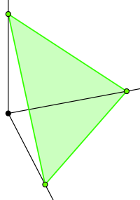
A probability density function on this surface can look like this when all of the faces are equally likely:
pdf <- function(v) ddirichlet(v, c(5, 5, 5))
mesh <- simplex_mesh(.0025) %>% as.data.frame %>% tbl_df
mesh$pdf <- mesh %>% apply(1, function(v) pdf(bary2simp(v)))

ggplot(mesh, aes(x, y)) +
  geom_raster(aes(fill = pdf)) +
  coord_equal(xlim = c(0,1), ylim = c(0, .85))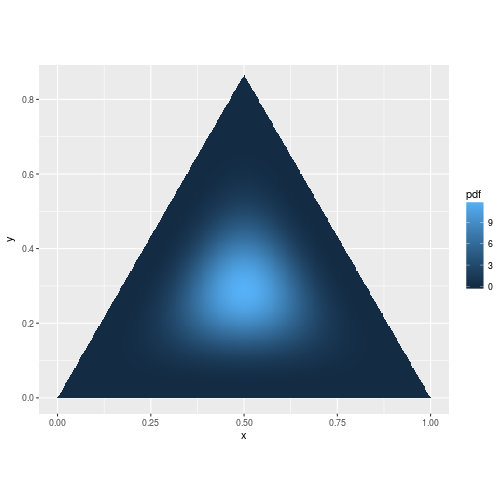
As we update our Dirichlet distribution using the rules above, it can shift the probability just like we saw for the beta distribution:
pdf <- function(v) ddirichlet(v, c(5, 5, 15))
mesh <- simplex_mesh(.0025) %>% as.data.frame %>% tbl_df
mesh$pdf <- mesh %>% apply(1, function(v) pdf(bary2simp(v)))

ggplot(mesh, aes(x, y)) +
  geom_raster(aes(fill = pdf)) +
  coord_equal(xlim = c(0,1), ylim = c(0, .85))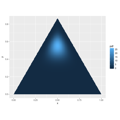
Unfortunately these visualizations don’t work so well for dice with more than three faces since it is hard to visualize probability densities in n-1 dimensions for an n-faced dice.
The Dirichlet distribution has a very similar form for the mean as the beta distribution for each of it’s dimensions $p_i$:
\[E[p_i] = \frac{\theta_i}{\sum_{i=1}^{k} \theta_i}\]In fact, if we were to just define $\beta$ as the sum of all the $\theta$s except $\theta_i$, and rename $\theta_i$ to $\alpha$, then the mean posterior probability for $\theta_i$ becomes indistinguishable from a beta distribution defined for $\theta_i$ and $\neg \theta_i$.
If we want the know a 95% credible interval for each face, then we can use this same trick to reduce each face of the dice to it’s own beta distribution and find the confidence interval for that. The only caveat to this is that we need to remember that the distributions for each p originally came from a Dirichlet distribution. This means that the condition that the sum of all p equal one still remains, and that if the true value for one of the p is actually lower than our posterior mean probability, then it is necessary that one or more of the other faces has a p higher than it’s posterior mean in an amount that cumulatively offsets the difference in the first p.
That’s enough theory. Let’s start analyzing!
Analysis
Rather than duplicating a bunch of code for each dice, I will just start by writing a function that can be reused. The parameters passed to the function are:
- roll_data: An integer vector containing the sequence of roll results.
- faces: The number of faces on the dice being analyzed
- beta_prior_a: The value of the alpha parameter to be used in the beta prior distribution
- beta_prior_b: The value of the beta parameter to be used in the beta prior distribution
bayesian_dice_analysis <- function(roll_data, faces = 20, beta_prior_a = 1, beta_prior_b = 1) {

  faces_start <- 1
  faces_sep <- 1

  # Deal with the d100. It has 10 faces starting at 0 instead of 1 and increasing in increments of 10.
  if (faces == 100) {
    roll_data <- as.numeric(roll_data)
    faces_start <- 0
    faces_sep <- 10
  }

  # Check that no rolls are non-numeric
  if (sum(is.na(roll_data)) > 0) {
    stop("Non-numeric rolls were found in the data. Please ensure that the data is valid.")
  }

  # Check that no rolls fall outside 1:faces
  if ((sum(roll_data > faces) + sum(roll_data < 0)) > 0) {
    stop(sprintf("Values outside the range 0 to %i were found in the data. Please ensure the faces parameter is correct and check that the data is valid.", faces))
  }

  # Check that alpha and beta are non-negative
  if (beta_prior_a < 0 || beta_prior_b < 0) {
    stop("The alpha and beta priors must both be non-negtive. Please ensure the values specified are correct.")
  }

  results_table <- tibble(face = seq(from = faces_start, to = faces_start + (faces - faces_sep), by = faces_sep))

  # Figure our the number of successes per face
  # Not sure how to do this inside a mutate function below
  successes <- c()
  for (i in results_table$face) {
    successes <- rbind(successes, sum(roll_data == i))
  }

  # Add columns for the count of binomial successes and failures
  results_table <- results_table %>%
    mutate(successes = successes,
           failures = length(roll_data) - successes)

  # Add the values related to the posterior distribution
  results_table <- results_table %>%
    mutate(beta_post_a = beta_prior_a + successes,
           beta_post_b = beta_prior_b + failures,
           posterior_mean = beta_post_a / (beta_post_a + beta_post_b),
           posterior_median = qbeta(0.5, beta_post_a, beta_post_b),
           posterior_mode = (beta_post_a - 1) / (beta_post_a + beta_post_b - 2),
           ci_95_lower = qbeta(0.025, beta_post_a, beta_post_b),
           ci_95_upper = qbeta(0.975, beta_post_a, beta_post_b))

  return(results_table)
}
The d10 dice is the one that I am really concerned about, so let’s start with it:
d10_data <- read_csv("d10.csv")
d10_result <- bayesian_dice_analysis(d10_data$Rolls, faces = 10, beta_prior_a = 10, beta_prior_b = 90)

ggplot(d10_result, aes(x = face, y = posterior_mean)) +
  geom_point() +
  geom_errorbar(aes(ymin = ci_95_lower, ymax = ci_95_upper), colour = "black", width = 0.1) +
  geom_hline(aes(yintercept = 0.10, color = "red")) +
  scale_x_continuous(breaks = round(seq(from = 0, to = 10, by = 1))) +
  theme(legend.position = "none") +
  coord_flip() +
  ggtitle("Posterior Probablities for Each Face of My d10 Dice") +
  labs(x = "Face of the Dice",
       y = "Posterior Probability Distribution")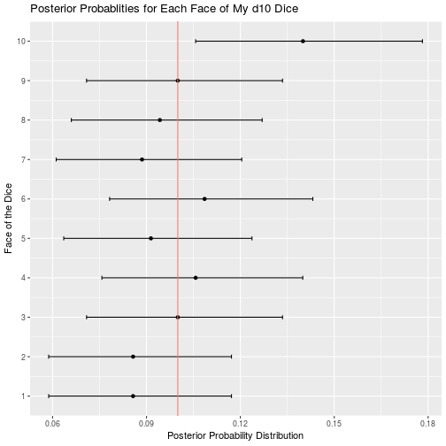
It definitely looks like my d10 is a little unbalanced, and in a favourable way for me. But it’s no where near as skewed as my reputation was leading me to believe. Based on the 95% credible interval the true probability of rolling a 10 is likely to found somewhere in the interval of approximately 0.105 to 0.180. This is certainly higher than 0.10, but no where near the “trick dice rolls 10 every time” levels I was concerned about. I think I’ll keep using the dice and hope that the DM never reads this blog post.
Out of curiosity, let’s analyze my other dice too:
d20_data <- read_csv("d20.csv")
d20_result <- bayesian_dice_analysis(d20_data$Rolls, faces = 20, beta_prior_a = 5, beta_prior_b = 95)

ggplot(d20_result, aes(x = face, y = posterior_mean)) +
  geom_point() +
  geom_errorbar(aes(ymin = ci_95_lower, ymax = ci_95_upper), colour = "black", width = 0.1) +
  geom_hline(aes(yintercept = 0.05, color = "red")) +
  scale_x_continuous(breaks = round(seq(from = 0, to = 20, by = 2))) +
  theme(legend.position = "none") +
  coord_flip() +
  ggtitle("Posterior Probablities for Each Face of My d20 Dice") +
  labs(x = "Face of the Dice",
       y = "Posterior Probability Distribution")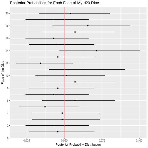
d12_data <- read_csv("d12.csv")
d12_result <- bayesian_dice_analysis(d12_data$Rolls, faces = 12, beta_prior_a = 100/12, beta_prior_b = 11 * 100/12)

ggplot(d12_result, aes(x = face, y = posterior_mean)) +
  geom_point() +
  geom_errorbar(aes(ymin = ci_95_lower, ymax = ci_95_upper), colour = "black", width = 0.1) +
  geom_hline(aes(yintercept = 1/12, color = "red")) +
  scale_x_continuous(breaks = round(seq(from = 0, to = 12, by = 1))) +
  theme(legend.position = "none") +
  coord_flip() +
  ggtitle("Posterior Probablities for Each Face of My d12 Dice") +
  labs(x = "Face of the Dice",
       y = "Posterior Probability Distribution")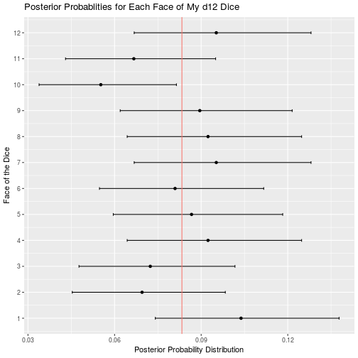
d100_data <- read_csv("d100.csv")
d100_result <- bayesian_dice_analysis(d100_data$Rolls, faces = 100, beta_prior_a = 100/10, beta_prior_b = 9 * 100/10)

ggplot(d100_result, aes(x = face, y = posterior_mean)) +
  geom_point() +
  geom_errorbar(aes(ymin = ci_95_lower, ymax = ci_95_upper), colour = "black", width = 0.1) +
  geom_hline(aes(yintercept = 1/10, color = "red")) +
  scale_x_continuous(breaks = round(seq(from = 0, to = 100, by = 10))) +
  theme(legend.position = "none") +
  coord_flip() +
  ggtitle("Posterior Probablities for Each Face of My d100 Dice") +
  labs(x = "Face of the Dice",
       y = "Posterior Probability Distribution")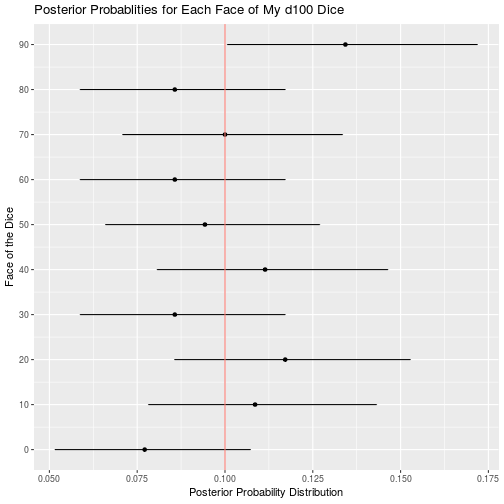
d8_data <- read_csv("d8.csv")
d8_result <- bayesian_dice_analysis(d8_data$Rolls, faces = 8, beta_prior_a = 100/8, beta_prior_b = 7 * 100/8)

ggplot(d8_result, aes(x = face, y = posterior_mean)) +
  geom_point() +
  geom_errorbar(aes(ymin = ci_95_lower, ymax = ci_95_upper), colour = "black", width = 0.1) +
  geom_hline(aes(yintercept = 1/8, color = "red")) +
  scale_x_continuous(breaks = round(seq(from = 0, to = 8, by = 1))) +
  theme(legend.position = "none") +
  coord_flip() +
  ggtitle("Posterior Probablities for Each Face of My d8 Dice") +
  labs(x = "Face of the Dice",
       y = "Posterior Probability Distribution")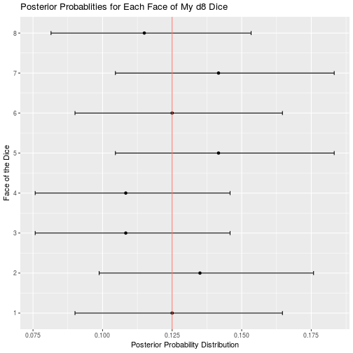
d6_data <- read_csv("d6.csv")
d6_result <- bayesian_dice_analysis(d6_data$Rolls, faces = 6, beta_prior_a = 100/6, beta_prior_b = 5 * 100/6)

ggplot(d6_result, aes(x = face, y = posterior_mean)) +
  geom_point() +
  geom_errorbar(aes(ymin = ci_95_lower, ymax = ci_95_upper), colour = "black", width = 0.1) +
  geom_hline(aes(yintercept = 1/6, color = "red")) +
  scale_x_continuous(breaks = round(seq(from = 0, to = 6, by = 1))) +
  theme(legend.position = "none") +
  coord_flip() +
  ggtitle("Posterior Probablities for Each Face of My d6 Dice") +
  labs(x = "Face of the Dice",
       y = "Posterior Probability Distribution")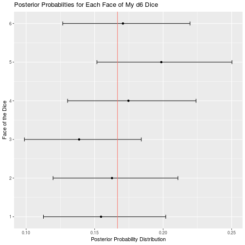
d4_data <- read_csv("d4.csv")
d4_result <- bayesian_dice_analysis(d4_data$Rolls, faces = 4, beta_prior_a = 100/4, beta_prior_b = 3 * 100/4)

ggplot(d4_result, aes(x = face, y = posterior_mean)) +
  geom_point() +
  geom_errorbar(aes(ymin = ci_95_lower, ymax = ci_95_upper), colour = "black", width = 0.1) +
  geom_hline(aes(yintercept = 1/4, color = "red")) +
  scale_x_continuous(breaks = round(seq(from = 0, to = 4, by = 1))) +
  theme(legend.position = "none") +
  coord_flip() +
  ggtitle("Posterior Probablities for Each Face of My d4 Dice") +
  labs(x = "Face of the Dice",
       y = "Posterior Probability Distribution")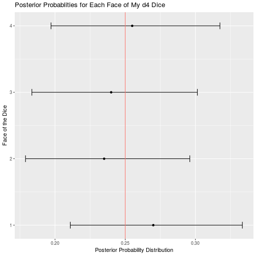
Of all my remaining dice, the only other potential issues are that my d12 may roll a 10 less than expected, and my d100 may roll 90 more that expected. I cannot think of a single time my character has had to roll a d12 so any unfairness in that dice is moot. Furthermore, a 10 is a good roll, so I will probably be disadvantaged by the balance issues in this dice. Similar to my d12, I rarely use my d100, so the benefits of rolling 90 more often than expected are wasted on my character. Overall my dice appear to be less than perfect, but I suppose that is to be expected when you order your dice in bulk from a generic looking amazon seller.