What Does my MNIST ConvNet Actually See?
Convolutional neural networks are powerful tools in the field of computer vision, and they tend to do very well at image recognition and classification tasks. Understanding why they work as well as they do can be a very daunting task however, especially when considering networks that do more than my toy MNIST example. Luckily the tools and techniques for visualizing ConvNet filters already exist, and should be easy to apply in this example. Almost all of the concepts and much of the code below is adapted from a blog post by Francois Chollet, the creator of the Keras library.
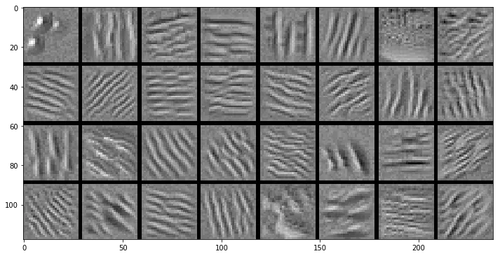
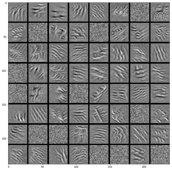
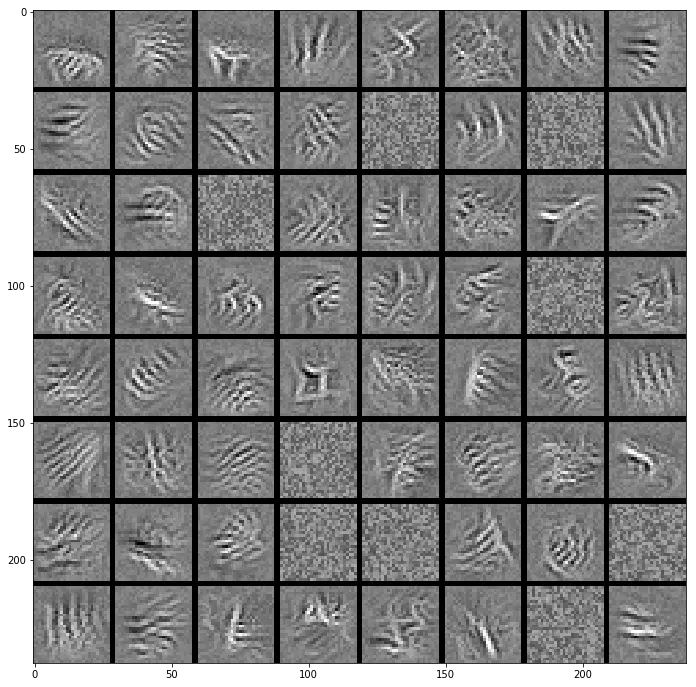
In my last post I created a convolutional neural network (ConvNet) using Keras and trained it on MNIST data for a Kaggle competition. This time I will create images for all of the filters in each of the four convolutional layers of that model, and then have the model generate the "perfect" version of each of the 10 digits it has been trained on. My hope is that this will help illuminate how the model goes about turning a bunch of messy pixels of human numeric digits in to nice clean digital representations.
from matplotlib import pyplot as plt
import numpy as np
import h5py
import keras
from keras.models import load_model
from keras import backend as K

# Set the matplotlib figure size
plt.rc('figure', figsize = (12.0, 12.0))

# Set the learning phase to false, the model is pre-trained.
K.set_learning_phase(False)
model = load_model('models/Jan-13-2018.hdf5')
# Figure out what keras named each of the layers in the model
layer_dict = dict([(layer.name, layer) for layer in model.layers])
print(layer_dict.keys())
dict_keys(['conv2d_1', 'conv2d_2', 'max_pooling2d_1', 'dropout_1', 'conv2d_3', 'conv2d_4', 'max_pooling2d_2', 'dropout_2', 'flatten_1', 'dense_1', 'dropout_3', 'dense_2', 'dropout_4', 'dense_3'])
# A placeholder for the input images
input_img = model.input

# Dimensions of the images
img_width = 28
img_height = 28

# A constant size step function for gradient ascent
def constant_step(total_steps, step, step_size = 1):
    return step_size

# Define an initial divisor and decay rate for a varied step function
# This function works better than constant step for the output layer
init_step_divisor = 100
decay = 10

def vary_step(total_steps, step):
    return (1.0 / (init_step_divisor + decay * step))
# Function from the Keras blog that normalizes and scales
# a filter before it is rendered as an image
def normalize_image(x):
    # Normalize tensor: center on 0., ensure std is 0.1
    x -= x.mean()
    x /= (x.std() + K.epsilon())
    x *= 0.1

    # Clip to [0, 1]
    x += 0.5
    x = np.clip(x, 0, 1)

    # Convert to grayscale image array
    x *= 255
    if K.image_data_format() == 'channels_first':
        x = x.transpose((1, 2, 0))
    x = np.clip(x, 0, 255).astype('uint8')
    return x
# Create a numpy array that represents the image of a filter
# in the passed layer output and loss functions. Based on the
# core parts of Francois Chollet's blog post.
def visualize_filter(layer_output, loss, steps = 256, step_fn = constant_step, input_initialization = 'random'):
    # Compute the gradient of the input picture wrt this loss
    grads = K.gradients(loss, input_img)[0]

    # Normalization trick: we normalize the gradient
    grads /= (K.sqrt(K.mean(K.square(grads))) + 1e-5)

    # This function returns the loss and grads given the input picture
    iterate = K.function([input_img], [loss, grads])

    if K.image_data_format() == 'channels_first':
        input_shape = (1, img_width, img_height)
    else:
        input_shape = (img_width, img_height, 1)

    # Initialize the input image. Random works well for the conv layers,
    # zeros works better for the output layer.
    input_img_data = np.random.random(input_shape) * 255.
    if input_initialization == "zeros":
        input_img_data = np.zeros(input_shape)
    input_img_data = np.array(input_img_data).reshape(1, 28, 28, 1)

    # Run gradient ascent for the specified number of steps
    for i in range(steps):
        loss_value, grads_value = iterate([input_img_data])
        input_img_data += grads_value * step_fn(steps, i)

    final_img = input_img_data[0]

    return final_img
# Define a function that stitches the 28 * 28 numpy arrays
# together into a collage of filters for each layer.
def stitch_filters(layer_filters, y_img_count, x_img_count):
    margin = 2
    width = y_img_count * img_width + (y_img_count - 1) * margin
    height = x_img_count * img_height + (x_img_count - 1) * margin
    stitched_filters = np.zeros((width, height))

    # Fill the picture with our saved filters
    for i in range(y_img_count):
        for j in range(x_img_count):
            img = layer_filters[i * x_img_count + j]
            stitched_filters[(img_width + margin) * i: (img_width + margin) * i + img_width,
                             (img_height + margin) * j: (img_height + margin) * j + img_height] = img

    return stitched_filters
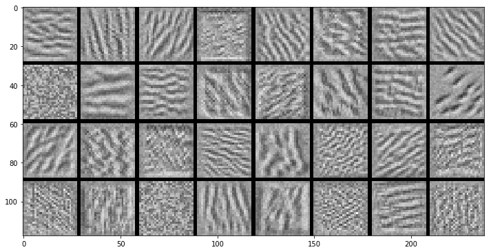
The First Convolutional Layer
# Start by visualizing the first convolutional layer
layer_name = 'conv2d_1'
layer_filters = []

# For each filter in this layer
for i in range(32):
    layer_output = layer_dict[layer_name].output
    loss = K.mean(layer_output[:, :, :, i])
    img = visualize_filter(layer_output, loss)
    layer_filters.append(img.reshape(28,28))

layer_filters = [normalize_image(image) for image in layer_filters]
layer_image = stitch_filters(layer_filters, 4, 8)

plt.imshow(layer_image, cmap = 'gray')
plt.show()
The Second Convolutional Layer
# The second convolutional layer
layer_name = 'conv2d_2'
layer_filters = []

# For each filter in this layer
for i in range(32):
    layer_output = layer_dict[layer_name].output
    loss = K.mean(layer_output[:, :, :, i])
    img = visualize_filter(layer_output, loss)
    layer_filters.append(img.reshape(28,28))

layer_filters = [normalize_image(image) for image in layer_filters]
layer_image = stitch_filters(layer_filters, 4, 8)

plt.imshow(layer_image, cmap = 'gray')
plt.show()
The Third Convolutional Layer
# The third convolutional layer
layer_name = 'conv2d_3'
layer_filters = []

# For each filter in this layer
for i in range(64):
    layer_output = layer_dict[layer_name].output
    loss = K.mean(layer_output[:, :, :, i])
    img = visualize_filter(layer_output, loss)
    layer_filters.append(img.reshape(28,28))

layer_filters = [normalize_image(image) for image in layer_filters]
layer_image = stitch_filters(layer_filters, 8, 8)

plt.imshow(layer_image, cmap = 'gray')
plt.show()
The Fourth Convolutional Layer
# The fourth layer
layer_name = 'conv2d_4'
layer_filters = []

# For each filter in this layer
for i in range(64):
    layer_output = layer_dict[layer_name].output
    loss = K.mean(layer_output[:, :, :, i])
    img = visualize_filter(layer_output, loss)
    layer_filters.append(img.reshape(28,28))

layer_filters = [normalize_image(image) for image in layer_filters]
layer_image = stitch_filters(layer_filters, 8, 8)

plt.imshow(layer_image, cmap = 'gray')
plt.show()
The Output Layer
# The final output layer of the model
output_filters = []

for i in range(10):
    output = model.output
    loss = K.mean(output[:, i])
    img = visualize_filter(output, loss,
                          steps = 4096,
                          step_fn = vary_step,
                          input_initialization = 'zeros')
    output_filters.append(img.reshape(28,28))

output_image_raw = stitch_filters(output_filters, 2, 5)

plt.imshow(output_image_raw, cmap = 'gray')
plt.show()
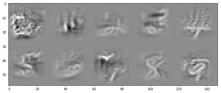
If you squint really hard, then the above images do sort of look like the digits they're meant to represent. The are very grey, however, which isn't at all like the original white on black MNIST digits provided. We can de-average the digits to restore them to a darker and less grey state:
# The above output filters are very grey, which isn't the way the
# original MNIST digits are represented.
def deaverage_digit(digit):
    deaveraged_digit = np.clip(digit - digit.mean(), 0, 255)
    deaveraged_digit *= (255.0/deaveraged_digit.max())
    return deaveraged_digit

deaveraged_outputs = [deaverage_digit(x) for x in output_filters]
output_image_deaveraged = stitch_filters(deaveraged_outputs, 2, 5)

plt.imshow(output_image_deaveraged, cmap = 'gray')
plt.show()
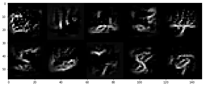
We can now make sure we computed things correctly by feeding these "perfect" digits back to the neural network for classification. If it doesn't return a correct classification for any of them, then we should probably suspect that something strange has happened.
# Make predictions on the output layer visualizations we just created
output_images = np.array(deaveraged_outputs).reshape(10,28,28,1)
predictions = np.argmax(model.predict(output_images), axis = 1)
print(predictions)
[0 1 2 3 4 5 6 7 8 9]
Everything checks out. It looks like the above images are good representations of what my MNIST convolutional neural network considers "perfect" for each digit. Ultimately it didn't do too terribly either; I can sort of recognize the digits myself. This probably has a lot to do with my prior knowledge of what each is supposed to represent though, and it might not go so well if I asked someone what each image was supposed to be without providing any context.
Still, it is reassuring that there are features in the above image that a human can recognize. In the blog post by Francois Chollet that inspired me to use these same techniques on my own model, it was found that the VGG16 (OxfordNet) model's idea of the perfect sea snake or perfect magpie looked nothing like what a human would consider either of those to be. My model has at least made it past the psychedelic patterns stage to where it looks like some proper abstraction is occurring in the final layer. This reassures me that it may not be completely over fit to the training data, and gives me a shred of hope that it will do well on the final private leader board scoring of the Kaggle MNIST digit recognition competition.