Hockey Modeling - Less Code, More Math! (Part 2)
This post is part of a series exploring the math behind my hockey model:
- Incorporating win/loss data for inference
- Predicting regulation score probabilities
- Predicting the winner in overtime/shootout
- Differentiating overtime wins from shootout wins
With Bayesian posterior distributions for the model parameters, we need to account for the full range of each when we go to estimate things like scores and win probabilities. We turn to probability theory and calculus to figure this out! Here we will see how to find the probabilities for different regulation time scores.
The probabilities of different regulation scores for each team
One of the key assumptions of my model is that the chance of one team scoring is independent of the current score, or the other team's chances of scoring. This means we can model the final score of the given team as a Poisson distributed random variable dependent only on that team's rate parameter $\lambda$.
Recall from an earlier post on this model that the Poisson rate parameters for each team are defined as:
$$log\lambda_{H,t} = i + h + o_{j,t} - d_{k,t}$$
$$log\lambda_{A,t} = i + o_{k,t} - d_{j,t}$$
$$ \lambda_{H,t} = exp(log\lambda_{H,t})$$
$$ \lambda_{A,t} = exp(log\lambda_{A,t})$$
Where each of $i$, $h$, $o_{:,t}$ and $d_{:,t}$ are approximated as normal random variables. The distribution for the sum of normal random variables is itself normal, giving us:
$$log\lambda_{H,t} \sim Normal(\mu_i + \mu_h + \mu_{o_{j,t}} - \mu_{d_{k,t}}, \sigma^2_i + \sigma^2_h + \sigma^2_{o_{j,t}} + \sigma^2_{d_{k,t}})$$
$$log\lambda_{A,t} \sim Normal(\mu_i + \mu_{o_{k,t}} - \mu_{d_{j,t}}, \sigma^2_i + \sigma^2_{o_{k,t}} +\sigma^2_{d_{j,t}})$$
The probability mass function (PMF) for the Poisson distribution says the probability that our team of interest scores $k$ goals in regulation time will be:
$$Pr(k|\lambda) = \frac{\lambda^{k} e^{-\lambda}}{k!}$$
Of course we don't have a single value for $\lambda$, but rather the log-normally distributed $\lambda_{H,t}$ and $\lambda_{A,t}$. In order to account for this we need to find the contribution of each possible value of $log\lambda$ to the probability of observing $k$ goals. We need to combine the Probability Density Function (PDF) of $log\lambda$ and the Poisson PMF. Since $log\lambda$ is normally distributed, its PDF is:
$$Pr(x|\mu, \sigma) = \frac{1}{\sigma \sqrt{ 2\pi}} exp \left(-\frac{1}{2} (\frac{x - \mu}{\sigma})^2 \right)$$
Now the trick to combining the Poisson PMF and Normal PDF is a bit of calculus. Let us represent a specific value of $log\lambda$ from its PDF as $x$. We then need to integrate over all possible values of $x$, finding both the probability of $x$ occurring, as well as the probability of $k$ goals given that $x$. This gives us:
$$Pr(k|\lambda \sim N(\mu, \sigma)) = \int_{\infty}^{-\infty} \frac{e^{xk} e^{-{e^x}}}{k!} \frac{1}{\sigma \sqrt{ 2\pi}} exp \left(-\frac{1}{2} (\frac{x - \mu}{\sigma})^2 \right) dx$$
Where $\mu$ and $\sigma$ are determined according to the definitions for $log\lambda_{H,t}$ and $log\lambda_{A,t}$ above. Note that this looks like a pretty tricky integral, and I'm not aware of any way to solve it analytically. That's why this blog post is titled Less Code, not No Code! We will solve this integral numerically using a method called Quadrature which the SciPy team has kindly implemented for us.
def bayesian_poisson_pdf(μ, σ, max_y=10):
    def integrand(x, y, σ, μ):
        pois = (np.exp(x)**y)*np.exp(-np.exp(x))/factorial(y)
        norm = np.exp(-0.5*((x-μ)/σ)**2.0)/(σ * sqrt(2.0*pi))
        return  pois * norm

    lwr = -3.0
    upr = 5.0

    y = np.arange(0,max_y)
    p = []
    for yi in y:
        I = quad(integrand, lwr, upr, args=(yi,σ,μ))
        p.append(I[0])
    p.append(1.0 - sum(p))

    return p
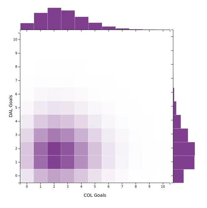
Once again, the assumption of independence has a major role to play. To find the regulation time scores for each game we simply iterate over each possible score $k$ for each team to get the marginal probabilities separately. Then the joint probability for a specific pair of scores is simply the product of the two marginal probabilities.
Everything above is what makes my regulation time score distribution plots work. For example, in tonight's game between Colorado and Dallas, we have the following predictions:
