Convolutional neural networks appear to be wildly successful at image recognition tasks, but they are far from perfect. They are known to be susceptible to attacks called adversarial examples, in which an image that is clearly of one class to a human observer can be modified in such a way that the neural network misclassifies it. In some cases, the necessary modifications may even be imperceptible to humans.

In this post we will explore the topic of adversrial examples using the Convolutional Neural Network I created for a Kaggle competition and then later visualized. To do so I will use the hand drawn digits that the neural network used as a validation set during training, and show that the neural network correctly classifies them 99.74% of the time. I will then use a library called CleverHans to compute adversarial examples that cause this accuracy to plummet. Finally I will introduce 10 brand new digits that I have drawn myself and show that they are classified correctly with high confidence. I will then try to compute perturbations that push the model into classifying each of these new example digits into each of the other nine possible digits. These perturbed examples will be visualized to show that the changes required for misclassification are often not as significant as you might expect.

from sklearn.model_selection import train_test_split
import pandas as pd

import numpy as np
import keras
from keras import backend
from keras.models import load_model
import tensorflow as tf

from cleverhans.attacks import FastGradientMethod
from cleverhans.attacks import BasicIterativeMethod
from cleverhans.utils_keras import KerasModelWrapper

from matplotlib import pyplot as plt
import imageio

# Set the matplotlib figure size
plt.rc('figure', figsize = (12.0, 12.0))

# Set the learning phase to false, the model is pre-trained.
backend.set_learning_phase(False)
keras_model = load_model('models/Jan-13-2018.hdf5')

/home/everett/.local/lib/python3.6/site-packages/h5py/__init__.py:36: FutureWarning: Conversion of the second argument of issubdtype from `float` to `np.floating` is deprecated. In future, it will be treated as `np.float64 == np.dtype(float).type`.
  from ._conv import register_converters as _register_converters
Using TensorFlow backend.
/usr/lib/python3.6/importlib/_bootstrap.py:219: RuntimeWarning: compiletime version 3.5 of module 'tensorflow.python.framework.fast_tensor_util' does not match runtime version 3.6
  return f(*args, **kwds)

'''
Split the provided training data to create a new training
data set and a new validation data set. These will be used
or hyper-parameter tuning.
'''

# Use the same seed to get the same validation set
seed = 27

raw_data = pd.read_csv("input/train.csv")
train, validate = train_test_split(raw_data, 
                                   test_size=0.1,
                                   random_state = seed, 
                                   stratify = raw_data['label'])

# Split into input (X) and output (Y) variables
x_validation = validate.values[:,1:].reshape(4200,28,28, 1)
y_validation = validate.values[:,0]

With the validation set that was used in training my MNIST Convnet, we can verify that the validation accuracy is actually 99.74% like expected.

# Set TF random seed to improve reproducibility
tf.set_random_seed(1234)

if not hasattr(backend, "tf"):
    raise RuntimeError("This tutorial requires keras to be configured"
                       " to use the TensorFlow backend.")

if keras.backend.image_dim_ordering() != 'tf':
    keras.backend.set_image_dim_ordering('tf')
    print("INFO: '~/.keras/keras.json' sets 'image_dim_ordering' to "
          "'th', temporarily setting to 'tf'")

# Retrieve the tensorflow session
sess =  backend.get_session()

# Define input TF placeholder
x = tf.placeholder(tf.float32, shape=(None, 28, 28, 1))
y = tf.placeholder(tf.float32, shape=(None, 10))

# Evaluate the model's accuracy on the validation data used in training
x_validation = x_validation.astype('float32')
x_validation /= 255

pred = np.argmax(keras_model.predict(x_validation), axis = 1)
acc =  np.mean(np.equal(pred, y_validation))

print("The normal validation accuracy is: {}".format(acc))

The normal validation accuracy is: 0.9973809523809524

Now we want to see if CleverHans is working. To do so we will initialize the FastGradientMethod attack object, which uses the Fast Gradient Sign Method (FGSM) to generate adversarial examples. The parameters used in this attack are exactly the same as those provided in the keras tutorial on the CleverHans GitHub Repo. We’ll then create the adversarial examples based on the validation data and check the classification accuracy.

# Initialize the Fast Gradient Sign Method (FGSM) attack object and 
# use it to create adversarial examples as numpy arrays.
wrap = KerasModelWrapper(keras_model)
fgsm = FastGradientMethod(wrap, sess=sess)
fgsm_params = {'eps': 0.3,
               'clip_min': 0.,
               'clip_max': 1.}
adv_x = fgsm.generate_np(x_validation, **fgsm_params)

adv_pred = np.argmax(keras_model.predict(adv_x), axis = 1)
adv_acc =  np.mean(np.equal(adv_pred, y_validation))

print("The adversarial validation accuracy is: {}".format(adv_acc))

The adversarial validation accuracy is: 0.2007142857142857

The classification accuracy has dropped from a respectable 99.74% to just 20.07% using a FGSM attack. This is one of the simplest adversarial attack methods available, and I expect that better results are possible with more sophisticated methods.

To get a feel for what the FGSM attack has done, let’s visualize one of the digits beside the corresponding adversarial example:

# Define a function that stitches the 28 * 28 numpy arrays
# together into a collage.
def stitch_images(images, y_img_count, x_img_count, margin = 2):
    
    # Dimensions of the images
    img_width = images[0].shape[0]
    img_height = images[0].shape[1]
    
    width = y_img_count * img_width + (y_img_count - 1) * margin
    height = x_img_count * img_height + (x_img_count - 1) * margin
    stitched_images = np.zeros((width, height, 3))

    # Fill the picture with our saved filters
    for i in range(y_img_count):
        for j in range(x_img_count):
            img = images[i * x_img_count + j]
            if len(img.shape) == 2:
                img = np.dstack([img] * 3)
            stitched_images[(img_width + margin) * i: (img_width + margin) * i + img_width,
                            (img_height + margin) * j: (img_height + margin) * j + img_height, :] = img

    return stitched_images

x_sample = x_validation[0].reshape(28, 28)
adv_x_sample = adv_x[0].reshape(28, 28)

adv_comparison = stitch_images([x_sample, adv_x_sample], 1, 2)

plt.imshow(adv_comparison)
plt.show()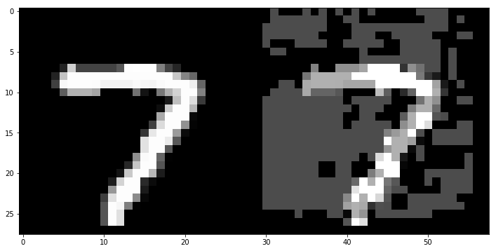

normal_digit_img = x_sample.reshape(1, 28, 28, 1)
adv_digit_img = adv_x_sample.reshape(1, 28, 28, 1)

normal_digit_pred = np.argmax(keras_model.predict(normal_digit_img), axis = 1)
adv_digit_pred = np.argmax(keras_model.predict(adv_digit_img), axis = 1)

print('The normal digit is predicted to be a {}'.format(normal_digit_pred))
print('The adversarial example digit is predicted to be an {}'.format(adv_digit_pred))

The normal digit is predicted to be a [7]
The adversarial example digit is predicted to be an [8]

The attack has perturbed the normal classification from a 7, which is correct, to an 8, which is obviously not. I don’t expect that any competent human would mistake the second image for an 8. The attack wasn’t imperceptible, so they may question why there appears to be a bunch of white noise in the image, but if pressed to identify the digit I am confident that nearly everyone will answer that it’s a 7.

Now let’s consider the 10 brand new digits I have created for this exercise. Each of these digits was drawn in Inkscape using a Wacom tablet. I then exported the svg files to a 28 x 28 pixel png image and inverted the colors to get white digits on a black background, just like the original MNIST data my model used.

# Load the new hand drawn digits from file
new_digits = []

for i in range(10):
    im = imageio.imread('input/new_digits/{}.png'.format(i))
    new_digits.append(im[:, :, 0] / 255.)

new_digits_img = stitch_images(new_digits, 1, 10)

plt.imshow(new_digits_img)
plt.show()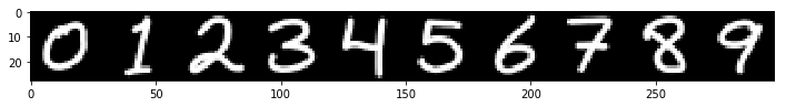

# Reshape the digits to the expected dimensions
new_inputs = np.array(new_digits).reshape(10,28,28,1)

# Check the accuracy 
conf = keras_model.predict(new_inputs)
pred = np.argmax(conf, axis = 1)
acc =  np.mean(np.equal(pred, np.array(range(10))))

print("The normal classifications are: {}".format(pred))
print("The normal classification confidences are: {}".format(conf.max(axis = 1)))
print("The normal classification accuracy is: {}".format(acc))

The normal classifications are: [0 1 2 3 4 5 6 7 8 9]
The normal classification confidences are: [1.         0.99881727 1.         1.         1.         0.99999976
 0.9999995  1.         1.         0.99999774]
The normal classification accuracy is: 1.0

My convnet does a fine job of identifying the new digits, correctly classifying each one with a minimum confidence of 99.88% on the one digit.

Now let’s see what happens when the examples are perturbed adversarially. This time we will use the Basic Iterative Method for attacks, which is an extension of the FGSM attack that can achieve misclassification with more subtle perturbations.

# Initialize the Basic Iterative Method (BIM) attack object and 
# use it to create adversarial examples as numpy arrays.
bim = BasicIterativeMethod(wrap, sess=sess)
bim_params = {'eps_iter': 0.01,
              'nb_iter': 100,
              'clip_min': 0.,
              'clip_max': 1.}
adv_x = bim.generate_np(new_inputs, **bim_params)
adv_conf = keras_model.predict(adv_x)
adv_pred = np.argmax(adv_conf, axis = 1)
adv_acc =  np.mean(np.equal(adv_pred, np.array(range(10))))

adv_list = np.split(adv_x, list(range(1,10)))
adv_list = [img.reshape(28,28) for img in adv_list]
adv_img = stitch_images(adv_list, 1, 10)

plt.imshow(adv_img, cmap = 'gray')
plt.show()

print("The adversarial classifications are: {}".format(adv_pred))
print("The adversarial classification confidences are: {}".format(adv_conf.max(axis = 1)))
print("The adversarial classification accuracy is: {}".format(adv_acc))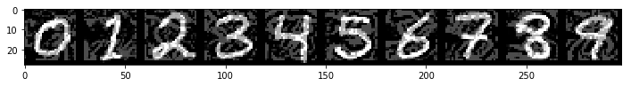

The adversarial classifications are: [9 2 8 8 8 3 8 8 3 8]
The adversarial classification confidences are: [0.9999982  1.         1.         1.         0.99999964 1.
 1.         1.         1.         1.        ]
The adversarial classification accuracy is: 0.0

The classification accuracy on the adversarial versions of the new digits has dropped to 0% and my convnet is alarmingly confident in these misclassifications. This time the minimum confidence is for the zero digit, which it has predicted is a nine with 99.99982% confidence. Once again, I do not expect any competent human being to make a similar mistake on the above examples.

Clearly my MNIST convnet is susceptible to adversarial examples, which isn’t surprising given that it was never trained on data that resembles these attacks. It is effectively over-fit to normal looking images of digits that were created in good faith, and adversarial examples expose this over-fitting in a dramatic fashion.

An important thing to note, however, is that the above attacks aren’t targeted towards a specific misclassification; it simply moves towards the easiest misclassification that it can find. A malicious actor might find more utility in forcing a specific misclassification if they intended to exploit my neural network in the real world. Let’s now consider how susceptible my convnet is to targeted adversarial attacks.

# Take a label and convert it to a one-hot vector
def labels_to_output_layer(labels):
    layers = np.zeros((len(labels), 10))
    layers[np.arange(len(labels)), labels] = 1
    return layers

# Take an image in the form of a numpy array and return it with a coloured border
def add_border(digit_img, border_color = 'black', margin = 1):
    digit_shape = digit_img.shape
    base = np.zeros((digit_shape[0] + 2 * margin, digit_shape[1] + 2 * margin, 3))
    rgb_digit = np.dstack([digit_img] * 3)
    
    if border_color == 'red':
        base[:,:,0] = 1
    elif border_color == 'green':
        base[:,:,1] = 1
    elif border_color == 'yellow':
        base[:,:,0] = 1
        base[:,:,1] = 1
    
    border_digit = base
    border_digit[margin:(digit_shape[0] + 1), margin:(digit_shape[1] + 1), :] = rgb_digit
    
    return base

# Attempt to perturb the input_digit to be misclassified as each of the target digits
# and return the resulting images with colored borders to indicate success or failure
def target_attacks(input_digit, input_digit_img, target_digits):
    
    results = []
    bim = BasicIterativeMethod(wrap, sess = sess)
    
    for target_digit in target_digits:
        border_color = 'black'
        output_layer = labels_to_output_layer([target_digit])
        bim_params = {'eps_iter': 0.01,
                      'nb_iter': 100,
                      'y_target': output_layer,
                      'clip_min': 0.,
                      'clip_max': 1.}
        adv_digit = bim.generate_np(input_digit_img, **bim_params)
        adv_pred = np.argmax(keras_model.predict(adv_digit), axis = 1)

        if adv_pred[0] == input_digit:
            border_color = 'green'
        elif adv_pred[0] == target_digit:
            border_color = 'red'
        else:
            border_color = 'yellow'

        adv_digit_img = add_border(adv_digit.reshape(28,28), border_color)

        results.append(adv_digit_img)
        
    return results

# For each of the ten digits, attempt to perturb it to the other nine
rows = []

for i in range(10):
    results = target_attacks(i, new_inputs[i].reshape(1,28,28,1), list(range(10)))
    results = [add_border(new_inputs[i])] + results
    results_img = stitch_images(results, 1, 11, margin = 0)
    rows.append(results_img)

# Add a final row for the target digits
last_row = [np.zeros((28,28))] + new_digits
last_row = [add_border(digit) for digit in last_row]
last_row_img = stitch_images(last_row, 1, 11, margin = 0)

rows.append(last_row_img)
    
final_img = stitch_images(rows, 11, 1, margin = 0)

# Plot the resulting grid
plt.imshow(final_img)
plt.xticks([])
plt.xlabel("Target Digits")
plt.yticks([])
plt.ylabel("Input Digits")
plt.show()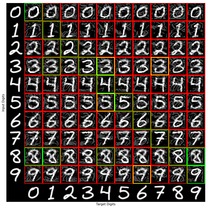

The first column in the above image represents the input digit, and the next ten digits on each row are attempts to perturb it into the digits zero through nine. The bottom row represents the target digit of the perturbation. A green border around a digit indicates that my convnet correctly classified the adversarial example as the original input digit, a red border means the digit was misclassified as the target digit, and a yellow border means the digit was misclassified, but not as the target. The diagonals are all correctly classified since they represent attempts to perturb a digit towards itself. We will not consider these diagonal entries when determining the accuracy of the model.

Counting the green digits off the diagonal, we can see that only five of the ninety attacks were correctly classified, and four more were misclassified as an unintended digit. Four of these five failed attacks are on the digit eight, suggesting that eights are not as easy as the other digits. Regardless, with 80 out of 90 attacks succeeding, we achieved a 88.9% success rate in forcing specific misclassications. It is no wonder adversarial examples have been such a topic of interest in machine learning circles over the past few years.

Now that I know my MNIST convnet is susceptible to adversarial attacks it might be interesting to try a similar technique while treating my network like a black box. To do this I would need to construct a parallel model which is used to find adversarial attacks that are likely to work on the original black box model. Such attacks are known to work in practice, and there is even a CleverHans tutorial that implements one. I might also try to improve this model by incorporating adversarial examples during training. Or I could instead switch to using the new Capsule Networks introduced only a few months ago by Geoffrey Hinton. Capsule Networks purport to be more resistant to adversarial examples due to the way in which they encode certain features like position, size, orientation, and stroke thickness. It will be interesting to see just how resilient they are against targeted attacks as time passes.